
The Revolutionary Paradigm of Quantum Computing
Welcome to the new quantum realm! Unlike traditional computing, which relies on binary bits (0s and 1s), quantum computing introduces qubits—tiny powerhouses that exist in multiple states at once, thanks to superposition.
In this blog, we’ll dive into the fundamentals of quantum computing with a simple “Hello World” program. Let’s explore how qubits break the rules of classical computing and open up a whole new world of possibilities!
Classical vs. Quantum Computing
The Classical Method
In conventional computing, each bit is either a 0 or a 1, similar to how a typical coin lands on heads or tails.
The Quantum Method
In the quantum domain, a qubit can exist as both 0 and 1 simultaneously, much like a spinning coin. This phenomenon, called superposition, enables quantum computers to evaluate multiple possibilities concurrently.
A Quantum Chess Analogy
Imagine you’re playing chess:
- Classical Computer: Evaluates moves one at a time, attempting various strategies through trial and error.
- Quantum Computer: Assesses all potential moves at once, courtesy of superposition, exponentially accelerating decision-making.
Writing "Hello World" in Quantum
Below is a basic Quantum Hello World program crafted in Microsoft’s Q# quantum programming language.
namespace QuantumProgram {
    open Microsoft.Quantum.Diagnostics;
    open Microsoft.Quantum.Intrinsic;

    @EntryPoint()
    operation Main() : Result {
        Message("Hello world!");
        use qubit = Qubit();
        // Apply a Hadamard gate to set the qubit in superposition
        H(qubit);
        // Measure the qubit (50% chance of 0 or 1)
        let result = M(qubit);
        // Reset the qubit before releasing it
        Reset(qubit);
        return result;
    }
}
Code Breakdown
- Initialize a Qubit: It begins in state |0>.
- Apply Hadamard Gate (H Gate): This places the qubit into a superposition of |0> and |1>.
- Measure the Qubit: The quantum state collapses to either |0> or |1>, with a 50% probability for each.
- Output the Result: You will see either 0 or 1 displayed.
Why the Random Output?
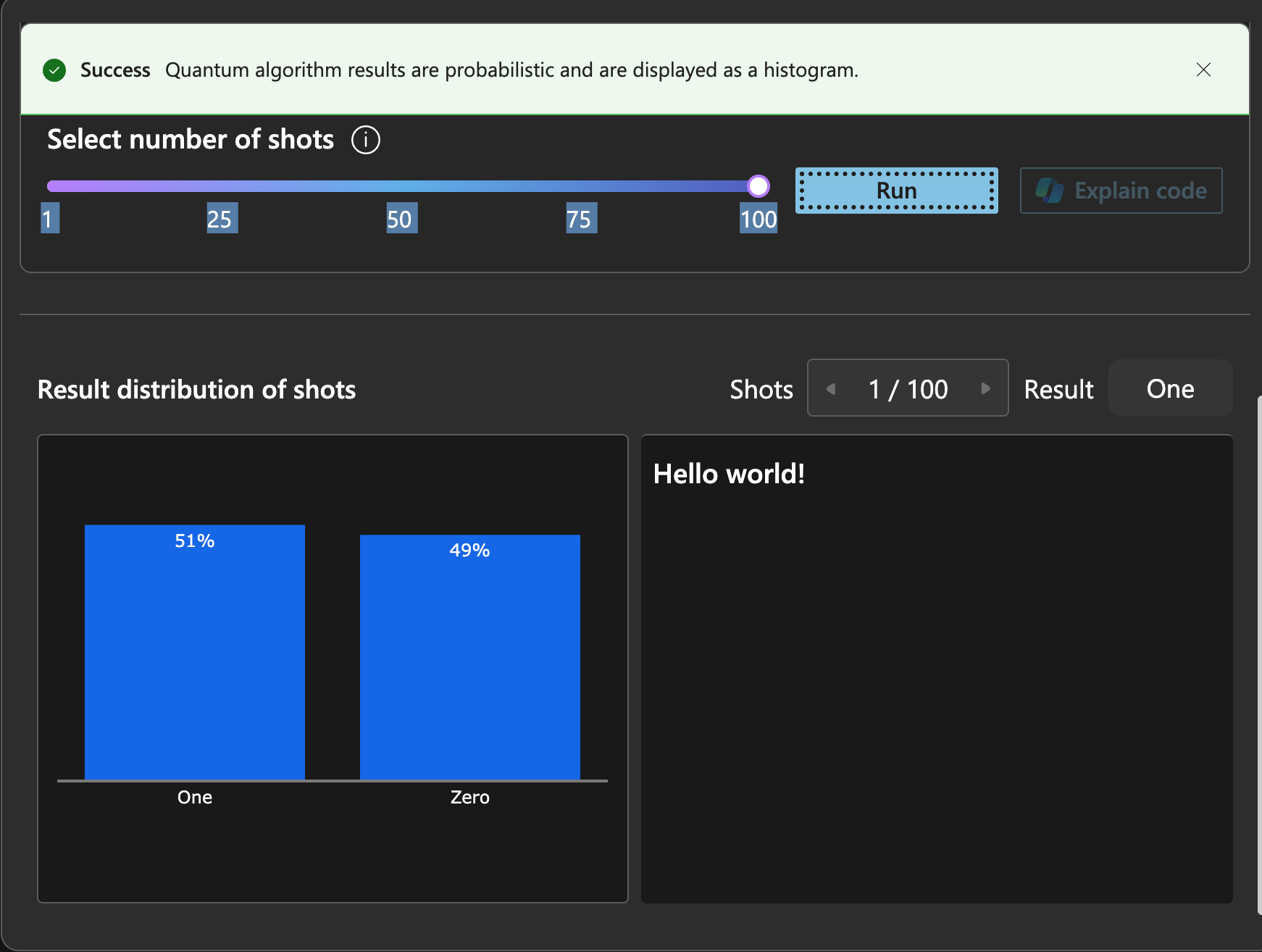
Running this program multiple times (say, 100 runs) would typically yield about 50% of results as 0 and the other 50% as 1. This randomness stems from quantum computing's probabilistic nature, contrasting with the deterministic nature of classical computing.
Quantum vs. Classical Math
Consider a simple calculation like 2 + 1:
- Classical Computer: The result is invariably 3.
- Quantum Computer: Due to superposition and quantum noise, the result isn’t always fixed. In some iterations, 2 + 1 might unexpectedly yield 6 due to its probabilistic nature.
Conclusion
Quantum computing introduces a radically different means of information processing. Our “Hello World” example illustrates:
- Superposition: Where qubits can exist across multiple states.
- Probabilistic Measurement: Making quantum outcomes inherently variable.
- Quantum Operations: Affecting calculations distinctly when compared to classical computing.
What’s Next?
In the next blog post, we will delve into advanced quantum operations and explore how qubits interact to resolve complex problems more swiftly than classical computers.
Stay tuned as we explore further into the quantum world!